Dow Theory Update for February 16: Does the Dow Theory work when applied to US bonds? (I)

Answer: YES!

This is a long post that took a good deal of research. If you want to become convinced about the Dow Theory being arguably the best timing system for trades lasting more than six months, continue reading.

Dow Theorist Hamilton stated that the Dow Theory could be applied to other markets. However, he did not put into practice his insight. As far as I am aware, no Dow Theorist followed Hamilton’s hint.

In these three posts, I proved that the Dow Theory could be successfully applied to gold/silver and GDX/SIL. There was outperformance in all markets and a marked drawdown reduction versus Buy and Hold (B&H):

http://www.dowtheoryinvestment.com/2021/06/dow-theory-special-issue-assessing-dow.html

http://www.dowtheoryinvestment.com/2021/06/dow-theory-special-issue-assessing-dow_15.html

http://www.dowtheoryinvestment.com/2021/06/dow-theory-special-issue-assessing-dow_24.html

Now is the turn for US bonds. Does the Dow Theory work when applied to US bonds? This answer is: YES.

I know many readers will be thinking: “I don’t care about such markets, much less precious metals as I am not a gold bug”. I respectfully answer: If you want to succeed using the Dow Theory or any other system, you must fully be convinced that it works. Conviction brings courage and consistency. Even if you only use it for stocks (or bonds, which is a larger market than stocks), you must be sure it works in other markets, as it is proof of its robustness. I’d be leery if the Dow Theory only worked when applied to US stock indexes. So, even if you disdain other markets, you need to know that the Dow Theory equally works. You need conviction as to its solidity. Knowledge breeds conviction.

Caveat: Unlike precious metals and their miners (our US stock indexes in thedowtheory.com), not all trades used in assessing the Dow Theory applied to US bonds were taken “life” on my blog. I’ve been covering TLT/IEF on a steady basis since 2018. Before that year, I haphazardly published about them on this blog.

I have used the “shorter-term” version of the Dow Theory; namely, I felt not bound by the three weeks’ time requirement usually accepted as a dogma to signal a secondary reaction. Nor felt I bound by the 1/3 retracement dogma. More about the “short-term” and “long-term” interpretation of the Dow Theory here.

As I explained on this Dow Theory blog, the three weeks’ time requirement and 1/3 retracement dogmas are based on a flawed interpretation of what Robert Rhea did. I debunked both misunderstandings here, here, and here.

Therefore, it is legitimate, logical, and feasible to free oneself from the strictures imposed by a flawed interpretation of the Dow Theory. Go and read what Rhea did. Not what other people say he did.

As you know, the concept of secondary reaction against the primary trend is vital for the Dow Theory. The highs/lows of secondary reaction serve as our pivot points to be broken out to signal a primary bull/bear market.

My rules have been the following:

1.      It is “classical” Dow Theory freed from the 1/3 retracement and three-week requirements.

2.      I require ten confirmed days as the time needed for a secondary reaction to exist. Exception: if there is a vast movement (i.e., March 2020), I may settle with a minimum of 5 confirmed trading days.

3.      I require that the movement exceeds the Volatility-Adjusted Minimum Movement (VAMM). In other words, if the minimum movement for US stock indexes is 3%, I multiply 3% times the ratio between TLT or IEF and the SPX. Let’s imagine the ratio is 0.8, so our VAMM would be 3 x 0.8 =2.4%.

4.      Since the Dow Theory requires two assets to have confirmation, I used TLT and IEF to appraise the trend.

5.      Start capital: USD 10,000

              

So, I feel my rules are very objective and can be replicated. No black-box.

 

Readers of this blog know that I usually trade a 50% position in each asset. I allocate an equal portion if I apply the Dow Theory to GLD/SLV or GDX/SIL. By doing this, I can never be too right or too wrong in case one of the two assets significantly underperforms. We also diversify across several ETFs when investing in US stock indexes (SPY, RSP, and DIA). We will study the addition of QQQ to the mix in a future post of this Dow Theory blog. However, when it comes to US interest rates, I don’t commit 50% of my trading equity to IEF due to its very low volatility and low potential profits (Example if Buy and Hold IEF yields 1.5% p.a., just guessing, and the Dow Theory results in 3% p.a. there is outperformance, but we remain with meager results due to IEF’s low volatility). Thus, I invest 100% in TLT.

 

EDV,  which is longer-term (30 years), is another ETF one may consider as it has wider swings and has more profit opportunities (and loss, if the downside is not taken care of) than TLT.

 

Since EDV’s inception date is 12/06/2007, the test starts on 12/26/2007 (closest primary bear market low to next Buy signal). Please mind that to compare Buy & Hold (B&H) performance v. the Dow Theory, we need to evaluate the performance between bottoms. So the start date is the bottom before the first Dow Theory Buy signal, and the end date is the bottom following the last Sell signal. Since one does not know when the bottom has been made until the next Buy signal comes, the test ends on 10/11/2021 (the last primary bear market low we know for sure, as the current one may go down further)—more details concerning the proper assessment of performance in this post.

 

I coded all the signals into TradeStation®. What follows is the computerized results. So let’s start with TLT. 

 

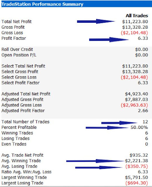
The first arrow shows net profit was $11,223, which is 112.23% performance, as the start capital was $ 10,000. B&H resulted in a mere 56.48%. The Dow Theory netted out a compounded annual return of 5.6032%. B&H only 3.2971%. In other words, the Dow Theory increased the yearly return by 69.94% v. B&H (2.3061 percentage points additional annual performance v. B&H)

The second arrow shows the profit factor (PF). The PF is the ratio between gross profit (money won) and gross loss (money lost in losing trades). The PF is a whopping 6.33, which means that for each $1 lost, we make $6.33. The secular bull market helped score such a high PF; however, the outperformance attests that the Dow Theory managed to add value. A high PF reflects the ability to “time trends.” The higher the figure, the more we catch the upside and avoid the downside.

The third arrow displays the total number of round trades taken: 12. Given that our test spans ca. 14 years, we can see that the “shorter-term” version of the Dow Theory does not result in overtrading.

The fourth arrow shows the percentage of winning trades: 50%. Investors should get this reality into their heads: it is unnecessary to win in most trades to succeed. One only needs to make more money when right (“let your profits run”) and cut losses short. The Dow Theory is, IMHO, one of the best trend following methods at cutting losses short without compromising the accuracy (measured by a high PF). Any trend following system can contain losses by placing tight stop-losses. However, the tighter the stop, the more the accuracy will degrade, and PF will decline. This is not the case with the Dow Theory. More about Dow Theory stop-losses in this old post. This is why I stopped reporting about the outcome of any given trade taken on this blog. The result of any given trade is immaterial, as it is like flipping a coin. Only when we have a string of trades (which under the Dow Theory means waiting for several years) does a picture of profits emerge.

The fifth and sixth arrows display the average winning and losing trade. As you can see, the average amount won in winning trades exceeds the average amount lost in losing trades by a factor of 6.33 (not a typo, the win/loss ratio equals by chance the PF).

The seventh arrow highlights the largest winning and losing trade. Even the largest losing trade is kept under control (ca. 7%).

Now let’s look at the figures below:

 

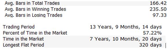
We observe that the average trade is slightly more than six months (166 bars =trading days). More interesting, we see that winning trades lasted an average of almost one year (235.5 bars close to 252 trading days=1 year), whereas losing trades lasted 4.4  months (97.33 bars). We see the axiom “cut your losses short” in action: Losing trades have a shorter lifespan than winning trades. Less time, lesser losses.

Noteworthy is the time in the market: 57.22%. Accordingly, 42.78% of the time, we were out of the market. This strengthens the Dow Theory outperformance v. B&H. The Dow Theory increased the annual return by 69.94% v. B&H by being in the market only 57.22% of the time. If we account for the missing time (69.94% increase in performance x 1.4278 -time out of the market-), we would be outperforming B&H by 100% (99.86%). Funds freed from trading bonds can be productively used in other markets (i.e., the stock market provided the trend, as appraised by the Dow Theory, is bullish too). The specifics of rotating between bonds and US stock indexes will be given in the future to our Subscribers. Here it suffices to say that going to stocks (in a bullish mode) when US bonds are bearish results in additional profits.

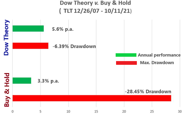
And what about drawdowns? Well, drawdown reduction is spectacular. For B&H, the deepest drawdown occurred between 12/19/2008 @122.26 to 4/5/2010 @87.47 for a total loss of -28.45%. For the Dow Theory, the deepest drawdown (closed trade basis) occurred from 3/13/2012 to 5/28/2008 for a total loss -of -6.39%. In other words, the drawdown was reduced by 77.5%. Please mind that even though the general tone of the market during the evaluated period was bullish, B&H had to endure several deep drawdowns.

Therefore, if we combine outperformance and drawdown reduction, the Dow Theory trounced B&H. Please remember that a drawdown reduction of, i.e., 50% is equivalent to double performance on a risk-adjusted basis. So both on absolute and risk-adjusted terms, the Dow Theory beat B&H.

This is nothing new. The same pattern of outperformance and risk reduction was proven to exist with precious metals and their ETF miners.

The following charts help you visualize the key figures:

 

If you think TLT’s outperformance and drawdown reduction was good enough, you’ve seen nothing yet. My next post will deal with the Dow Theory applied to the more volatile EDV, the long-term duration ETF. Until then, stay tuned.

Sincerely,

Manuel Blay

Editor of thedowtheory.com