Bull market for the gold and silver miners ETFs (GDX & SIL) signaled on 8/25/26

 

Overview: According to Dow Theory, the gold and silver miners ETFs, GDX and SIL, have turned bullish again. Gold and silver themselves, however, remain in a bullish secondary reaction and are still relatively far from triggering a new bull market signal. Nevertheless, my research shows that miners tend to lead the underlying metals, making their renewed strength a potentially encouraging sign.

General Remarks:

In this post, I provide an in-depth explanation of the rationale behind employing two alternative definitions to evaluate secondary reactions.

SIL refers to the Silver Miners ETF. More information about SIL can be found HERE.

GDX refers to the Gold Miners ETF. More information about GDX can be found HERE.

A) Market situation if one appraises secondary reactions not bound by the three weeks and 1/3 retracement dogma.  

As I explained in this post, the trend was signaled as bearish on 6/9/26.

Following the 7/20/26 lows there was a secondary (bullish) reaction against the bear market.

The rally was so strong that, without any meaningful pullback, it surpassed the previous secondary reaction highs (deep blue rectangles on the left in the charts below).

The rally was so strong that, without any meaningful pullback, it surpassed the previous secondary reaction highs (deep blue rectangles on the left in the charts below).

According to Dow Theory (Rhea’s book The Dow Theory, page 77), the breakup of the highs of the last completed secondary reaction serves as an alternative way to signal a new bull market (and, alternatively, the lows of the last completed secondary reaction serve as the relevant prices to monitor for a new bear market). You can get more information about this alternative signal HERE, HERE, and HERE.

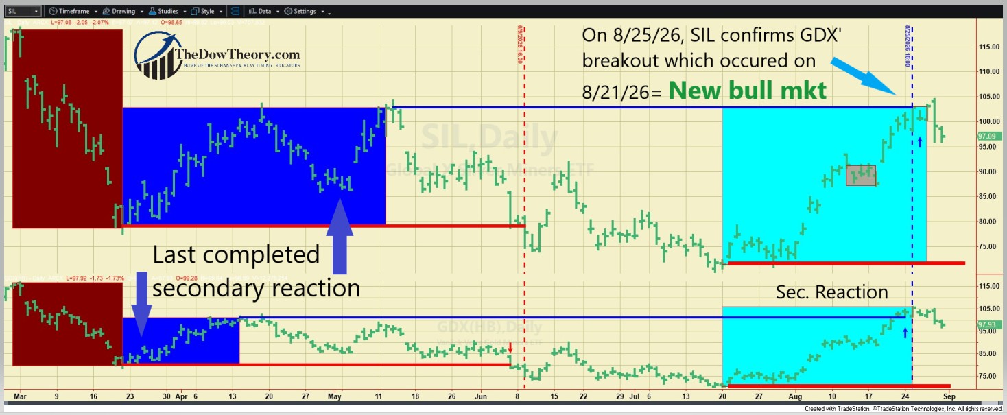
The charts below show the most recent price action: the deep blue rectangles on the left display the previously completed secondary reaction. Their respective closing highs, highlighted by the blue horizontal lines, were the hurdles both ETFs had to surpass for a new primary bull market signal. The light blue rectangles show the secondary reaction against the bear market, which, without any meaningful pullback, pushed higher until breaking above the highs of the previous secondary reaction. The thick red horizontal lines on the right of the charts show the last recorded bear market lows, which, if pierced by both ETFs, would signal a new bear market.

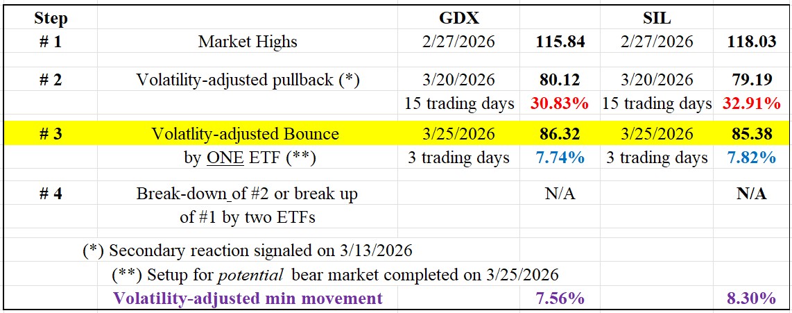
The table below gives you the relevant prices whose joint violation would signal a new bear market.

So, the primary and secondary trends are bullish.

B) Market situation if one sticks to the traditional interpretation demanding more than three weeks and 1/3 confirmed retracement to declare a secondary reaction.

As I explained in this post, the trend was signaled as bearish on 6/9/26.

In this instance, the longer-term application of Dow Theory yields the same result: the trend shifted to bullish on 8/25/26.

Sincerely,

Manuel Blay

Editor of thedowtheory.com

 

 

 

 

 

To Stop or Not to Stop: The Controversy

 

A Practical Framework For Managing Risk In Your Portfolio

A recent thread on X.com about stop losses turned into a small controversy, as this topic tends to do, because it quickly polarizes people. Here is the link to my post:

https://x.com/ManuelBlay3/status/2085467290200625336

 

On one side are those who insist you need a stop and that skipping one is simply reckless. On the other are those who consider a stop a tool for people who end up getting run by algorithms and market makers, placed exactly where everyone else’s stop already sits. What follows is a distillation of that back-and-forth, an attempt to bring some clarity to when a stop genuinely makes sense and when it does not, which depends entirely on your personal approach to trading and the strategy you are actually running.

Path One: Protection Through Breadth, Not Through Stop-Loss

If your edge is fundamental, meaning you are buying businesses because of earnings power, balance sheet quality, or a mispriced cash flow stream, a mechanical price stop is often the wrong tool. Fundamentals move slowly. A drawdown in a sound business is frequently noise rather than signal, and a rigid stop turns a temporary markdown into a realized loss right before the thesis has time to play out. The logical alternative is to buy on good fundamentals, give the trade time, and sell only when those fundamentals deteriorate. Applying a price-based stop in that context is not caution; it is self-sabotage.

The protection here comes from position count and position sizing, not from a stop loss rule. A portfolio of twenty stocks or more, reasonably sized and not concentrated in a single sector, already absorbs company-specific risk the way an index does. One name can fall sharply, and the portfolio survives.

This is also the honest answer to the sharpest objection raised in the discussion: whether rejecting stops means accepting a catastrophic loss from a surprise event such as a bad offering or an accounting scandal. It does not, provided the position was sized correctly in the first place. A severe loss on a name that was four or five percent of the portfolio is painful but survivable. A severe loss on a name that was the entire position is a different problem altogether, and no stop loss discussion fixes bad sizing after the fact.

There is a practical problem hiding inside this path, though, and it deserves to be said plainly rather than assumed away. Twenty stocks is the minimum for proper diversification, yet finding twenty genuinely attractive fundamental ideas through discretionary judgment alone is no easy task. How do you consistently decide what is good and what is bad? How much weight should be given to earnings, quality, value, momentum, or any of the other factors that matter? Most investors, working through annual reports, model one company at a time and run out of high conviction ideas well before they reach twenty. Depth of research and breadth of names pull against each other, and something usually gives: either the position count shrinks below what real diversification requires, or the quality of research per name thins out to fill the roster.

But if building a portfolio of twenty high-quality ideas is difficult, deciding when those same twenty stocks should be sold is even more challenging.

Buying is only half the battle. A company rarely goes from attractive to unattractive overnight, and determining when its fundamentals have deteriorated enough to justify a sale is often a matter of judgment rather than a clear-cut decision.

And this is precisely where human nature becomes dangerous.

I was reminded of this while reading the latest “Market Wizards” book. One trait appears again and again among even extraordinarily successful traders: learning to control risk was difficult. It wasn’t simply a matter of knowing that stops or exit rules were necessary. Even when traders had them, the temptation to override them was often there.

I recognize the problem because I experienced it myself. When I started trading, a stock could hit my stop, and I would think: let’s give it a little more room, it will recover. And the dangerous thing is that this often worked, maybe eight times out of ten. But the other two times, the stock didn’t recover. The loss kept compounding and eventually became enormous. Those few disasters could wipe out much of what had been gained from all the occasions when overriding the stop appeared to have been the correct decision.

The problem, therefore, is not merely designing an exit rule. The problem is obeying it.

The solution I have settled on is what I call “quantamentals”. The underlying inputs are still fundamental: growth, value, quality, profitability, earnings revisions, the same building blocks any fundamental investor would recognize, but they are processed on a quantified, computerized basis rather than judged name by name through memory, instinct, and conviction.

This approach solves two problems at once. First, it makes genuine diversification practical. Instead of developing twenty separate high-conviction narratives, the computer evaluates the entire investment universe using the same rules and ranks each stock accordingly. I don’t need twenty compelling stories. I need twenty stocks that objectively score better than the alternatives.

The second advantage may be even more important: quantification imposes discipline on the sell side. Every rebalance produces stocks that deserve to enter the portfolio and stocks that no longer deserve to remain in it. If five better-ranked stocks need to come in, cash must be raised by selling stocks whose rankings have deteriorated. That completely changes the psychology of selling.

There is no “let’s wait another week.”

No “maybe it will come back.”

No emotional attachment to the original thesis.

The rule for selling is not a price level; it is a rank-based exit. A position is sold when its “quantamental profile” deteriorates past a defined threshold, not when the story I originally told myself about the company stops feeling true. That distinction matters more than it sounds. A stock held because of a narrative gets defended long after the evidence has changed, because human beings are remarkably good at finding new reasons to defend an old decision. A stock held because of a quantified score has no story to defend. It has a ranking, and when that ranking deteriorates sufficiently, it goes.

I have come to think of the portfolio almost like the shelves of a supermarket. Shelf space is scarce. If some oranges are deteriorating while fresher, better merchandise is waiting to take their place, the supermarket owner does not become emotionally attached to the old oranges. He clears the shelf and replaces them.

A quantitative portfolio works much the same way. Capital is scarce shelf space. A stock does not need to become a disaster before it deserves to be sold. It merely needs to become less deserving of that scarce capital than the alternatives. This is a subtle but crucial difference: I am not necessarily selling because something terrible has happened to the company or because its price has crossed an arbitrary line, but because better opportunities now exist relative to the rest of the investment universe.

This is why, in a diversified quantitative strategy, risk management does not have to mean placing a mechanical stop beneath every position. Risk is controlled through small position sizes, diversification across sectors, systematic ranking, and the disciplined replacement of deteriorating holdings. The computer does not hope. It does not fall in love with a stock. And, most importantly, it does not second-guess the sell signal.

Jim Simons and Renaissance Technologies built the most successful track record in the industry, largely without discretionary stop-losses on individual positions. Their protection came from an entirely different architecture: thousands of small, statistically independent bets, each with a modest edge, held briefly, sized so that no single position could meaningfully damage the fund, and diversified across so many uncorrelated signals that the portfolio behaved closer to an insurance book than to a stock picker’s book. Risk was managed at the level of the whole system through position sizing, correlation control, and turnover, not at the level of any single trade’s exit price.

But some of you may still think that a stop loss would add an additional layer of protection to an already well-diversified portfolio based on “quantamentals”. I am sorry to disappoint you. The addition of stops to such strategies always results in a sharp degradation of performance.

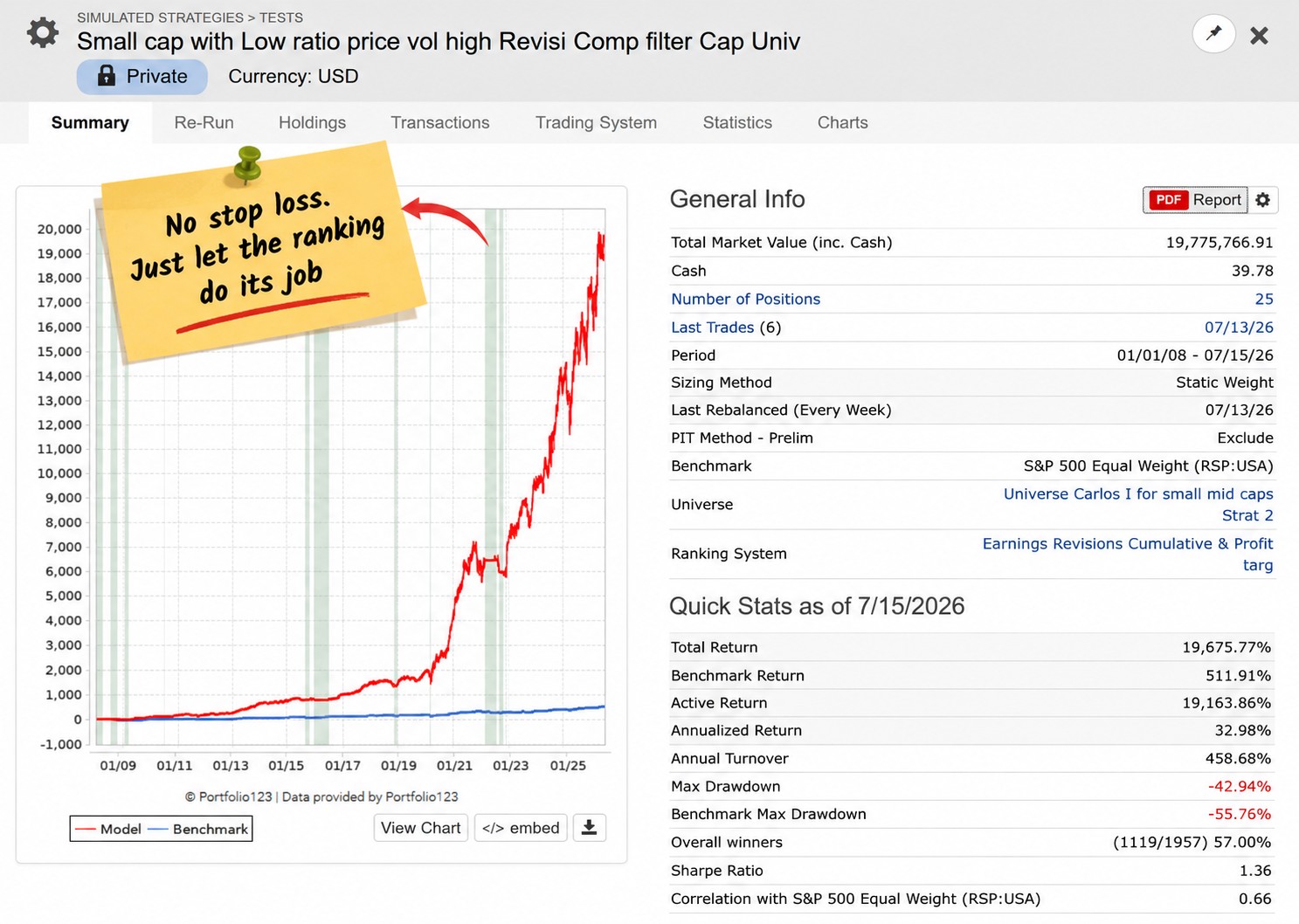
The image below shows one of my quant strategies without a stop-loss. A nice equity curve with an annual performance of 32.98% and a -42% drawdown.

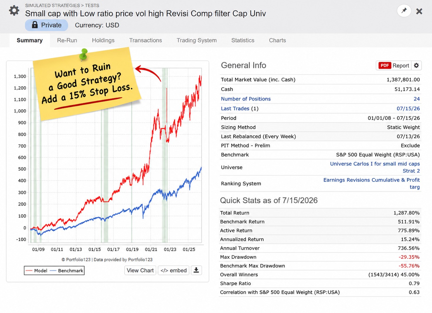
Now, if we add a 15% stop-loss, we effectively ruin the strategy, as the chart below shows. Performance is nearly halved, falling to 15.24%, while the maximum drawdown improves by only 31%, declining to 29.35%. This relatively modest reduction in drawdown comes at far too high a cost in performance.

The deterioration in risk-adjusted returns is equally striking: the Sharpe ratio falls from 1.36 without a stop loss to just 0.79 with the 15% stop.

Furthermore, turnover explodes to 736%, adding substantial transaction costs and slippage and making the strategy extremely difficult to trade in practice.

Therefore, if one invests based on “quantamentals”, one should steer away from using stop-losses.

Path Two: Protection Through The Stop-Loss

If instead your edge is technical, such as buying breakouts, moving-average crossovers, price patterns, or swing trading, and, to make things worse, you have few positions open at the same time, a stop is not optional. Furthermore, such “technical” traders tend to have a very concentrated portfolio, often with fewer than 5 positions. In such a case, a stop-loss is a vital tool for survival.

But not all stops are equal, and this is where many traders get it wrong. There are dummy stops and intelligent stops.

Dummy stops

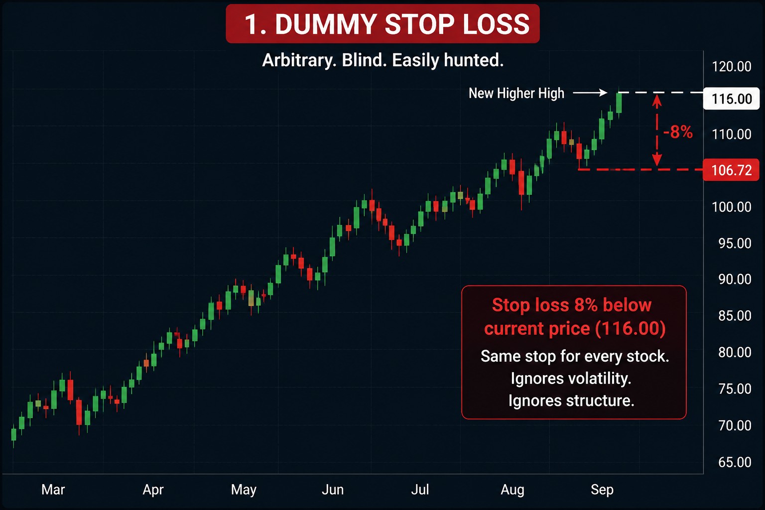
A dummy stop is an arbitrary number applied uniformly across every trade, most commonly a fixed percentage such as ten or fifteen percent below the purchase price, regardless of the stock, its volatility, or the chart. It is easy to implement, and it is also blind. A fixed percentage means almost nothing on a stock that regularly swings eight percent in a week, and it means far too much on a stable low-volatility name where that same move already signals something has genuinely broken.

Intelligent stops

An intelligent stop is derived from the security itself and/or context rather than imposed on it. Three layers are worth building, in increasing order of sophistication.

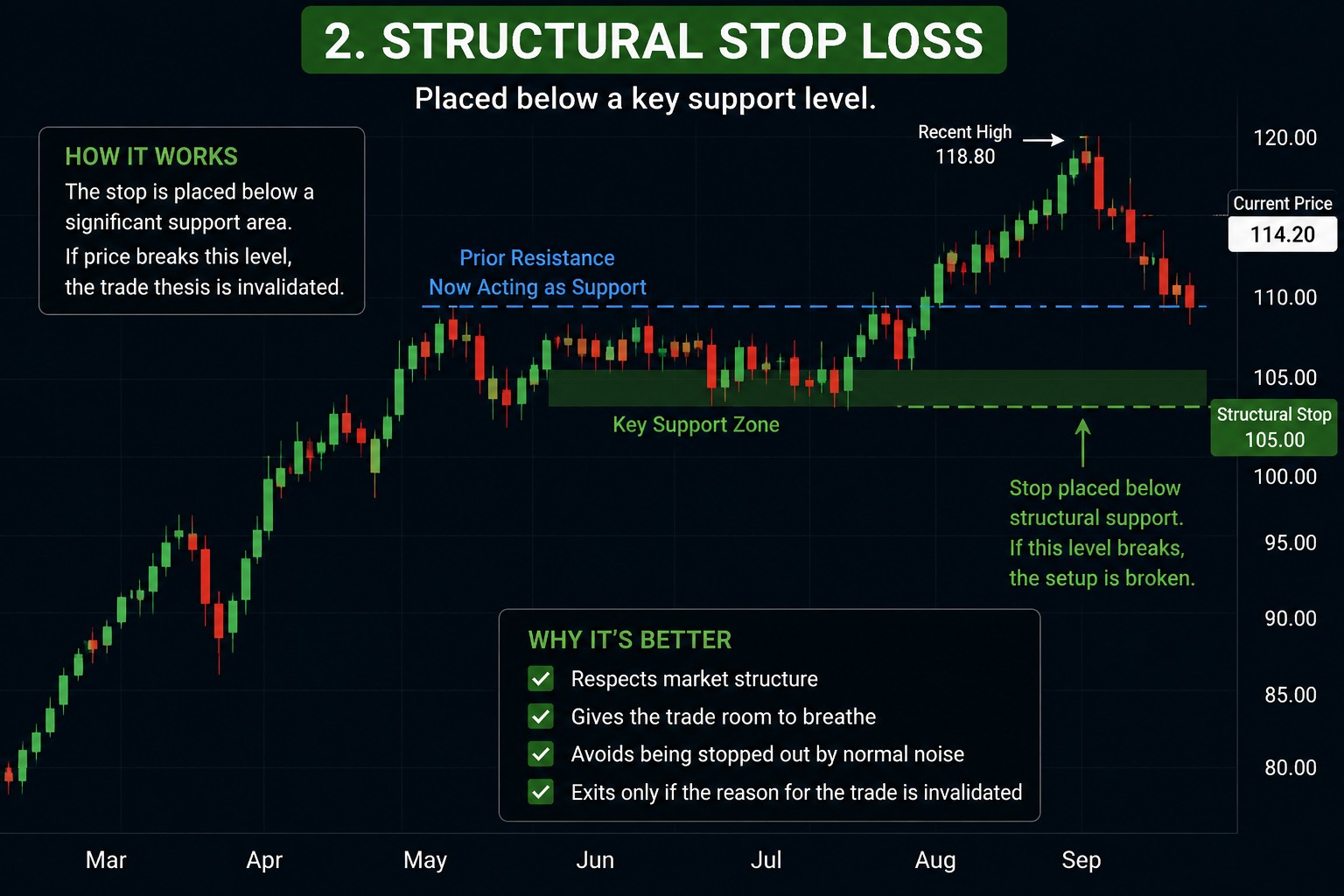
Structural or chart-based stops. A more discerning trader places the stop beneath a level that has actual meaning on the chart, a prior base, a broken resistance that should now act as support, or a key moving average such as the 50-day, the 150-day, or the 200-day line, chosen depending on the entry pattern. The logic is simple. If price falls back through the exact level that justified the trade, the original reason for owning the stock is no longer valid, and the position should be closed on its own merits rather than at an arbitrary distance.

 

One objection worth answering directly is the claim that placing a stop at an obvious technical level is pointless because everyone else’s stop sits at the same price, and that level gets run before the real move happens. There is truth in it. Round numbers, prior lows, and textbook moving averages are exactly where liquidity clusters, and price can and sometimes does push through a crowded level before reversing. The correct response to that is not to abandon technical stops; it is to stop placing them exactly on the obvious number. A volatility buffer below the structural level, or the confirmation requirement described above, both exist specifically to avoid being the easy liquidity at a level everyone can see on the same chart.

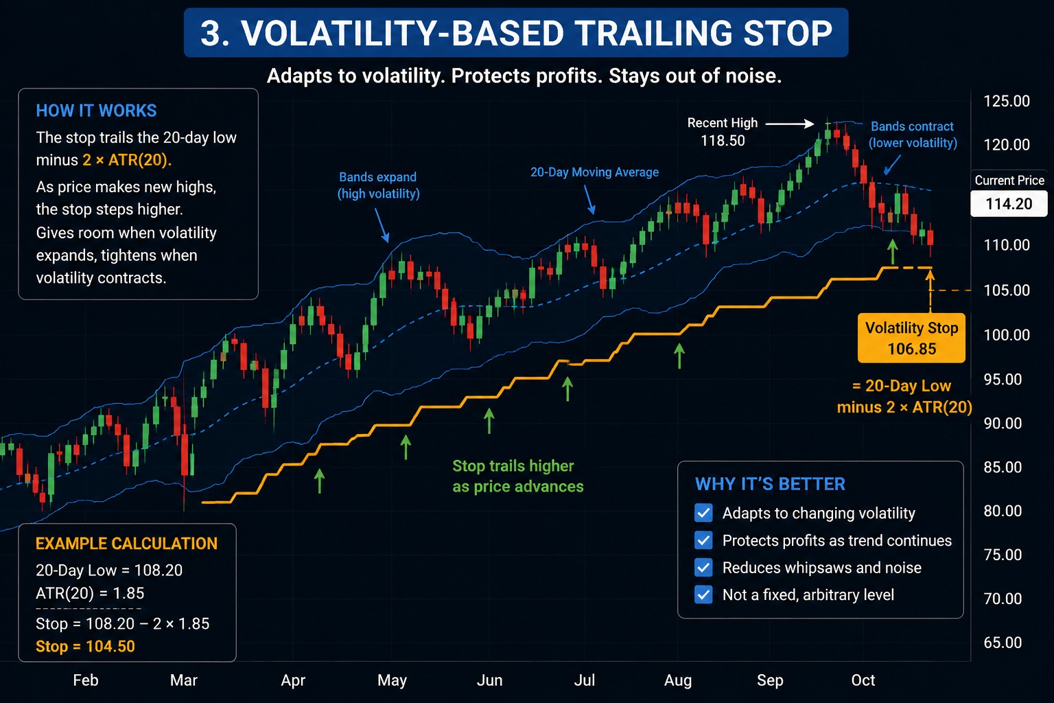
Volatility-based stops. Instead of a fixed percentage, the stop is set as a multiple of the stock’s own average true range or realized volatility, giving the best of both worlds, avoiding a premature exit on a normally noisy name while still keeping risk genuinely managed. A volatile name gets more room, a quiet name gets a tighter leash.

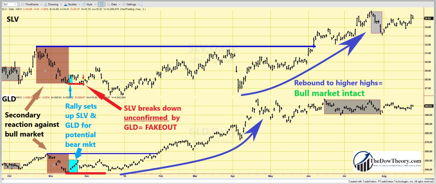
Confirmation-based stops. This is the most refined layer and the one closest to classical Dow Theory thinking. A single instrument breaking a significant technical level can be a fakeout, a stop run, or noise driven by low liquidity. Requiring confirmation from a related asset filters out a meaningful share of false signals. If the stock breaks its level but the related asset holds firm, the break is more likely noise. If the two assets break together, the signal is real, and the exit should follow without hesitation. This is the same principle that governs price and Advance Decline line confirmation in classical Dow Theory, applied here at the level of a single position’s exit rule.

The image below, whose full explanation you may find in this post, provides an excellent example of stops based on the principle of confirmation. The piercing of SLV (silver ETF) at a relevant low, unconfirmed by GLD (gold ETF), proved to be a fakeout.

The Third Path: The No Stop Fallacy For Day Traders

A different objection surfaces often in these threads: the claim that day traders do not need stops at all because closing every position before the close removes overnight gap risk entirely. This is true as far as it goes, and it is also close to the most unhelpful answer people give to the stop question, because it treats day trading as a fixed strategy rather than a capacity-constrained one.

A day trader working with a modest account is right that flattening at the close solves the gap problem, and there is nothing wrong with building a living around that approach. But day trading does not scale the way the argument implies. Executing meaningfully large size within a single session, without moving the price against yourself, becomes progressively harder as the deployed assets grow, because intraday liquidity in any single name is finite and a large order worked in a few hours leaves a visible footprint. The trader who is right to skip stops at a modest account size is not automatically right once that account reaches real scale, not because the logic about gaps changed, but because pure day trading stops being available at that size. Growing an account seriously eventually forces a longer time frame, and a longer time frame is exactly where the gap risk the argument dismissed comes back, along with the need for a genuine stop discipline.

Furthermore, day traders who trade without stop losses often overlook the fact that a stock can collapse dramatically even within a single trading session. If you run a highly concentrated portfolio, which is often the case with only three or four positions, a single stock falling 30% intraday can inflict catastrophic damage on your overall portfolio. In other words, the absence of overnight risk does not eliminate the need for risk management. Even over the course of a single day, concentrated positions can produce losses large enough to jeopardize an entire trading account.

The Weak Point Of Stop-Losses: The gap

If you trade a concentrated portfolio of a few stocks, the risk of one gapping down would be unbearable, rendering any stop-loss moot. This is a hidden risk for which there is no “standard” protection (unless you use puts or similar sophisticated hedging strategies). A stop-loss will not protect you against a stock that drops 60% overnight. The takeaway is clear: even if you are a technical trader for whom the stop-loss is a must, you must strive for a diversified portfolio.

I have a hard time understanding traders who brag about their “high conviction,” “focused” portfolio. In this game, the objective is survival. Survive, and performance will follow.

Choosing Your Path

The mistake to avoid is not picking the wrong philosophy; it is borrowing the confidence of one philosophy while practicing another. A concentrated breakout trader who refuses to use a stop because Renaissance did not use one is not being sophisticated; he is simply unprotected because he lacks the breadth of positions and the statistical edge that made the stopless approach survivable at scale. Equally, a diversified fundamental investor who panics into a tight mechanical stop on every position is importing a discipline built for a different game entirely.

The honest question to ask before every position is not, “What is my stop?” It is, which game am I playing, and does my protection actually match it?

Sincerely,

Manuel Blay

Editor of thedowtheory.com

 

 

Dow Theory Update for July 31: Primary Bear Market in U.S. Bonds Reaffirmed on 7/29/2026

 

The bear market in bonds continues

General Remarks:

In this post, I thoroughly explained the rationale behind my use of two alternative definitions to appraise secondary reactions.

TLT is the iShares 20 plus Years Treasury Bond ETF. More about it here.

IEF is the iShares 7 to 10 Years Treasury Bond ETF. More about it here.

Thus, TLT tracks longer term US bonds, whereas IEF tracks middle term US bonds. A bull market in bonds entails lower interest rates. A bear market in bonds represents higher interest rates.

A) Market situation if one appraises secondary reactions not bound by the three weeks and 1/3 retracement dogma.

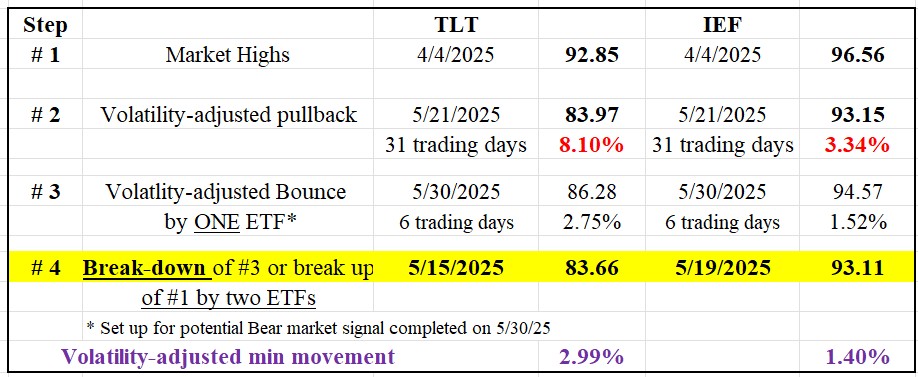
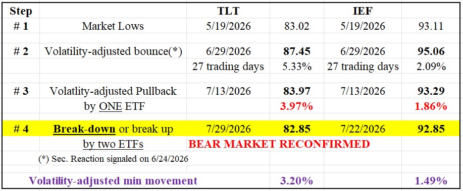
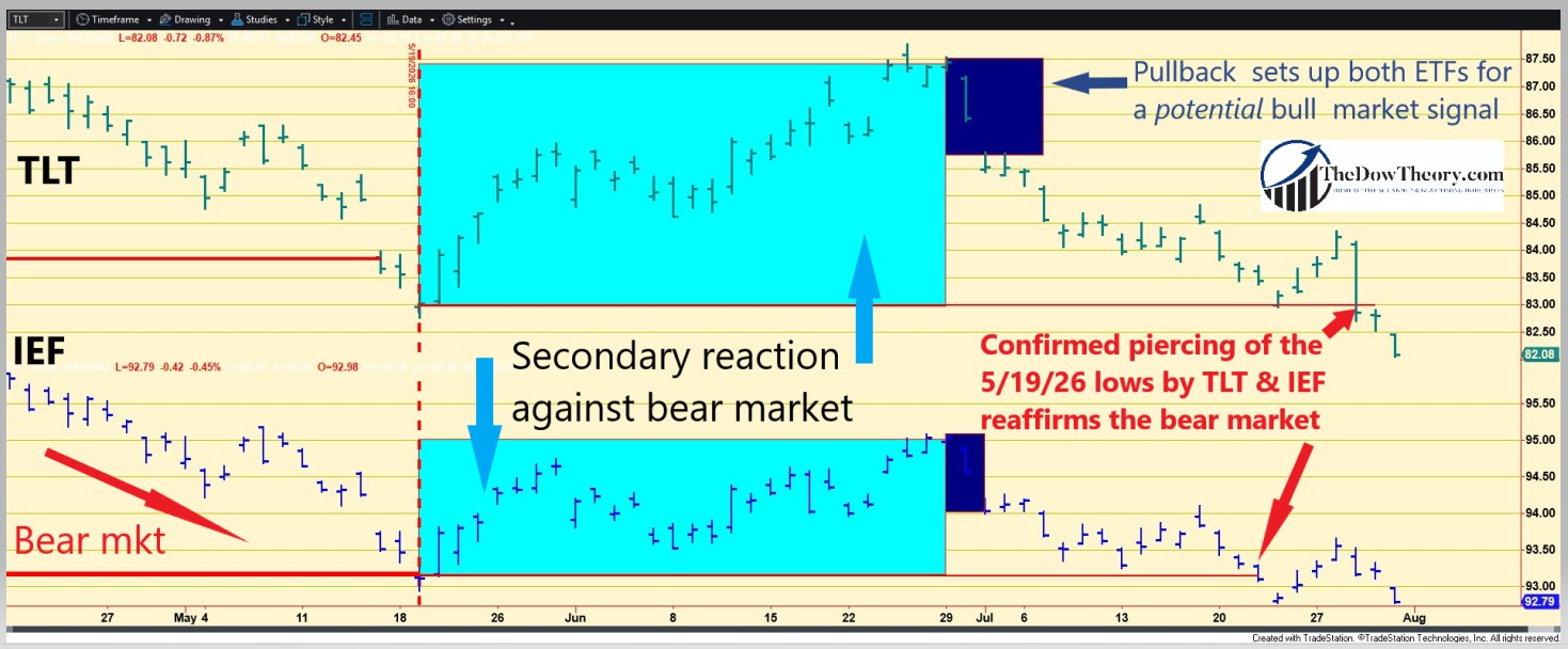
As I explained HERE, the primary trend was signaled as bearish on 5/19/2026. Following the 5/19/2026 bear market lows, a rally ensued, qualifying as a secondary (bullish) reaction against the primary bear market. The secondary reaction itself was signaled on 6/24/2026, and the volatility-adjusted bounce was completed on 6/29/2026, 27 trading days off the lows. Finally, a pullback on 7/13/2026 set up TLT and IEF for a potential primary bull market.

After the pullback, both ETFs headed lower over the following weeks. On 7/22/2026, IEF penetrated its 5/19/2026 primary bear market lows. On 7/29/2026, TLT broke down below its 5/19/2026 lows, providing confirmation. The Table below shows you the details:

So, the implications of the newer lows are as follows:

1) The secondary reaction against the primary bear market has been terminated. Now the secondary trend is also bearish.

2) The setup for a potential primary bull market has been canceled.

3) The primary bear market signaled on 5/19/2026 has been reaffirmed.

The charts provide a visual representation of price action in the market over the past few months, spanning from the lows observed on 5/19/2026 to the present day. The blue rectangles will indicate the secondary (bullish) reaction against the primary bear market. The dark blue rectangles represent the pullback that set up both ETFs for a potential primary bull market. The red horizontal lines will highlight the primary bear market lows of 5/19/2026, which have recently been pierced.

Therefore, it appears that the bond market continues to price in persistent inflationary pressure rather than the likelihood of an imminent recession. It is not necessarily a harbinger of a bear market in equities, but it may continue to limit their upside.

B) Market situation if one sticks to the traditional interpretation demanding more than three weeks and 1/3 confirmed retracement to declare a secondary reaction.

In this specific instance, the longer-term application of the Dow Theory aligns with the shorter-term rendering explained above. In other words, the price action and the Table shown above fully apply when we take the longer term view as well. Therefore, the primary trend shifted to bearish on 5/19/2026, and both the primary and secondary trends are bearish under this interpretation too.

Sincerely,

Manuel Blay

Editor of thedowtheory.com

 

The Closest Thing to a Free Lunch in Investing

 

The Magic of Combining Strategies

One of the advantages of quantitative investing is that diversification can be engineered rather than left to chance.

I run several independent quant strategies. Within each one, I impose a strict rule: no single sector may account for more than 30% of the portfolio. That limit prevents any individual strategy from becoming overly concentrated. Still, a 30% allocation to one sector can be meaningful and a tad too high to my taste.

This is where the real magic begins.

Instead of relying on a single strategy, I combine four different strategies, each with its own stock-selection logic and sector profile, allocating 25% of the capital to each. The result is far more balanced than any of the individual strategies alone.

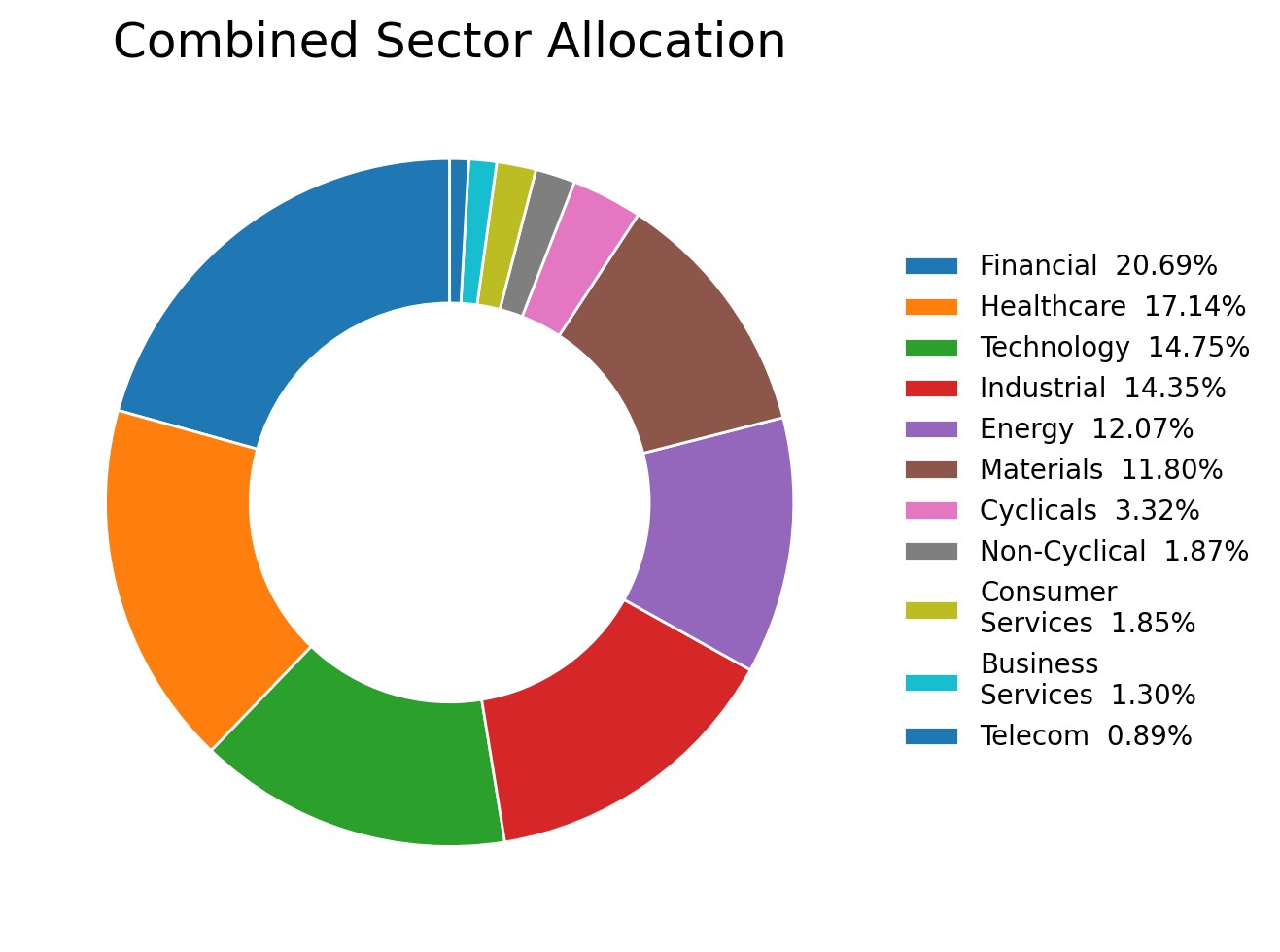
As the chart below illustrates, my current combined portfolio’s largest sector is Financials at just 20.69%, followed by Healthcare at 17.14%. No sector comes remotely close to the original 30% cap. The different strategies naturally offset one another, smoothing out sector concentrations without sacrificing their individual strengths.

The same phenomenon extends beyond sectors. The combined portfolio also achieves a healthier mix of market capitalizations while preserving its intended exposure to the mid and small- cap universe.

This is one of the closest things to a free lunch in investing: by combining multiple robust strategies that behave differently, you reduce concentration risk and build a more diversified portfolio without diluting the edge of the underlying models.

And yes, you guessed it: by combining the four strategies, volatility is reduced, as are the spells of underperformance vs. the benchmark.

Furthermore, I was recently asked whether I planned to incorporate AI or quantum computing stocks into my portfolios. My answer was very simple: if they offer a high probability of outperforming over the next three months, my system will find them, and they will automatically appear on my buy list.

That is one of the greatest advantages of a fully systematic, quantitative approach. I don’t have to spend my time trying to identify the next hidden gem or debating whether AI or quantum computing is the investment theme of the future. My job is simply to trust the process.

If AI or quantum stocks truly offer superior expected returns, my models will naturally allocate more capital to them within their respective sectors. If they don’t, they won’t make the cut. Rather than chasing narratives, I let my system do the work—and let the data make the decisions.

Sincerely,

Manuel Blay

Editor of thedowtheory.com

Some Lessons I Have Learned as a Quantitative Trader

 

Outperformance Comes in Bursts, Pain Comes in Stretches

What follows is based on my own experience as a quantitative trader. Other quants, using different models, different universes, or different constraints, may have reached different conclusions.

One of the first lessons I have learned is the importance of understanding the universe one is trading. I run one specific strategy focused on S&P 500 constituents, but most of my other strategies also include mid- and small-caps. I generally avoid microcaps because their low liquidity often makes backtests unrealistic and live trading difficult. It is very easy to produce extraordinary historical returns in illiquid stocks that cannot be replicated in the real world.

Even when I focus on relatively liquid small- and mid-caps with strong ranking profiles, the experience can be psychologically demanding. By ranking profile, I mean the relative attractiveness of a stock based on factors such as financial strength, business quality, growth, value, momentum, or a combination of several of these. In theory, a portfolio of highly ranked stocks should do well. In practice, the journey is rarely smooth.

What I have observed is that small and mid-caps often underperform the S&P 500 for extended periods. This can happen even when the strategy is fundamentally sound and has a strong long-term record. Over a two-year period, and often even over one year, my quantitative strategies have usually outperformed the S&P 500. But that outperformance does not usually come in a steady, comfortable way.

Instead, it often comes in bursts.

This is one of the most important lessons. A strategy may lag badly for months. You may see the S&P 500 rise 10% in five months while your own strategy is flat. That is not easy to endure. It feels as if something is wrong. It creates doubt. It tests your confidence in the model.

Then, suddenly, in a period of only six or eight weeks, the same strategy may gain 25% and leave the S&P 500 far behind. The brief burst of outperformance more than compensates for the long and frustrating period of underperformance.

This is why there is no free lunch. Quantitative strategies may deliver superior long-term results, but they demand psychological fortitude. It is not enough to have a good model. One must also have the temperament to stick with it when it is temporarily out of favor.

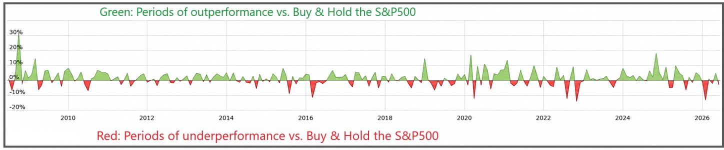
The screenshots below illustrate this point clearly. The first chart displays the periods of underperformance (in red) and outperformance (in green) of one of my quant-based trading strategies relative to a simple S&P 500 buy-and-hold approach.

What matters is not merely the final result. What matters is the path taken to get there. And the road may feel uncomfortable.

You can observe several spells of underperformance. In hindsight, they look tolerable. In real time, they are painful. They test your patience because you do not know whether the strategy is merely going through a normal bad stretch or whether something has genuinely stopped working.

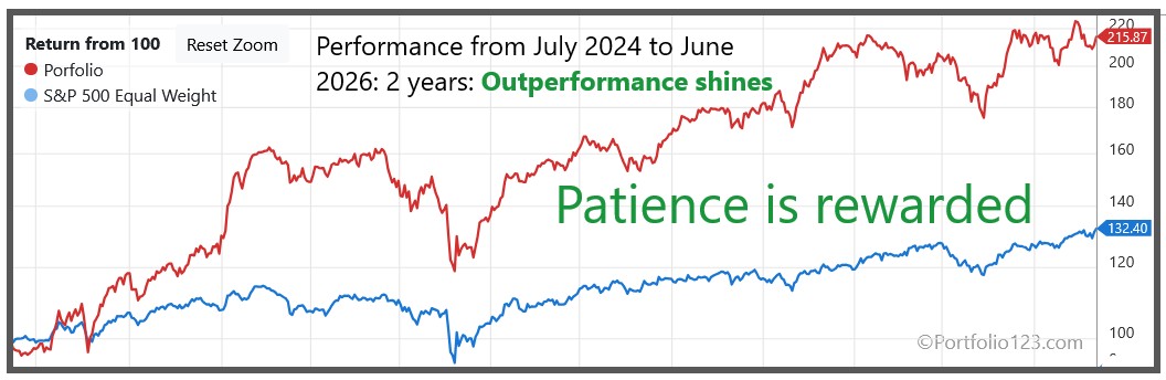
However, if we look back over two years, the picture changes completely, as shown in this chart:

The same strategy becomes a strong outperformer. And if we extend the view to almost 20 years, its long-term outperformance relative to the S&P 500 becomes even clearer.

Importantly, these results are not based on a frictionless theoretical exercise. A substantial slippage assumption of 0.25% per side of each trade has been included. That matters because, especially when trading smaller and mid-sized companies, ignoring slippage can make a strategy look much better on paper than it would have been in the real world.

The key takeaway is simple: patience is essential. The more your portfolio differs from the S&P 500, especially if it includes smaller companies, the more likely you are to underperform the index for extended periods. Your edge may not show up every month, or even every quarter. Often, it appears in short, powerful bursts that more than offset the painful spells of relative weakness.

That is the price of outperformance, and it is a price that can only be paid by those with the patience and psychological fortitude to stay the course when the going gets tough. In the end, that is often what separates the winners from the losers.

Sincerely,

Manuel Blay

Editor of thedowtheory.com

Gold and Silver miners ETFs Turn Bearish on 6/9/2026

 

Overview: In my June 1st Letter to subscribers, I noted that the two-year Treasury yield was breaking higher and that this would likely exert a negative influence on liquidity.

One of the main casualties appears to have been the gold and silver miners. On 6/9/26, a new bear market was signaled in both GDX and SIL. Gold and silver themselves have also been affected, as I discussed in this post.

Stocks, by contrast, have been affected only modestly so far. The decline has not even been enough to turn the secondary trend bearish. Therefore, both the primary and secondary trends for stocks remain bullish.

General Remarks:

In this post, I elaborate extensively on the rationale behind employing two alternative definitions to evaluate secondary reactions.

SIL refers to the Silver Miners ETF. More information about SIL can be found HERE.

GDX refers to the Gold Miners ETF. More information about GDX can be found HERE.

A) Market situation if one appraises secondary reactions not bound by the three weeks and 1/3 retracement dogma.  

As I explained in this post, the trend was signaled as bullish on 6/2/25.

Following a pullback (secondary reaction against the bullish trend), both GDX and SIL experienced a bounce, setting up both ETFs for a potential primary bear market signal. You can find detailed explanations and charts HERE.

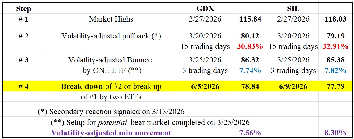
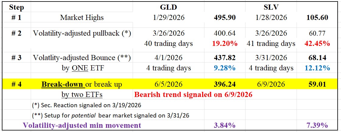
The table below gives you all the relevant information:

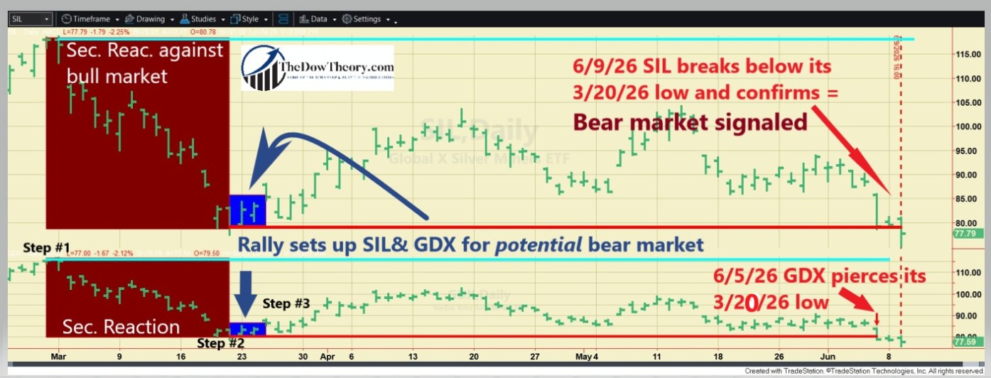
On 6/5/26, GDX broke down below its 3/20/26 pullback lows (Step #2). On 6/9/26, SIL confirmed by piercing its 3/20/26 closing lows. Since it was a confirmed violation, a primary bear market was signaled according to the Dow Theory.

Check out the chart below for a visual walkthrough of the recent price action. The brown rectangles highlight the secondary reaction (Step #2), the blue rectangles show the rally (Step #3) originating from the secondary reaction lows that set up both ETFs for a potential bear market signal, and the red horizontal lines pinpoint the pullback lows whose joint violation signaled the new bear market. The blue horizontal lines highlight the last recorded primary bull market highs (Step #1), whose upside breakout would signal a new primary bull market.

 

Thus, both the primary and secondary trends are currently bearish.

B) Market situation if one sticks to the traditional interpretation demanding more than three weeks and 1/3 confirmed retracement to declare a secondary reaction.

As I explained in this post, the trend was signaled as bullish on 6/2/25.

In this instance, the long-term application of the Dow Theory coincides with the shorter-term version, so there was a secondary reaction against the primary bull market, and the setup for a potential bear market signal has been completed. The confirmed violation of the 3/20/26 secondary reaction low triggered a bear market signal.

Thus, both the primary and secondary trends are currently bearish.

Sincerely,
Manuel Blay

Editor of thedowtheory.com

 

After a Long Ride, Gold and Silver Turn Bearish on 6/9/2026

 

Overview: In my June 1st Letter to subscribers, I noted that the two-year Treasury yield was breaking higher and that this would likely exert a negative influence on liquidity.

One of the main casualties appears to have been gold and silver. Today, 6/9/26, a new bear market was signaled in both metals. Gold and silver miners have also been hit, and I will address them in a separate post.

Stocks, by contrast, have been affected only modestly so far. The decline has not even been enough to turn the secondary trend bearish. Therefore, both the primary and secondary trends for stocks remain bullish.

General Remarks:

In this post, I extensively elaborate on the rationale behind employing two alternative definitions to evaluate secondary reactions.

GLD refers to the SPDR® Gold Shares (NYSEArca: GLD®). More information about GLD can be found HERE.

SLV refers to the iShares Silver Trust (NYSEArca: SLV®). More information about SLV can be found HERE.

A) Market situation if one appraises secondary reactions not bound by the three weeks and 1/3 retracement dogma.  

As I explained in this post, the primary trend was signaled as bullish on 4/2/24.

Following a pullback (secondary reaction against the bullish trend), both GLD and SLV experienced a bounce, setting up both ETFs for a potential primary bear market. You can find detailed explanations and charts HERE.

The table below gives you all the relevant information:

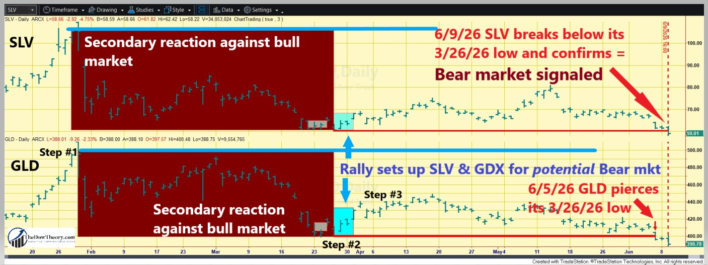
On 6/5/26, GLD broke down below its 3/26/26 pullback lows (Step #2). On 6/9/26, SLV confirmed by piercing its 3/26/26 closing lows. Since it was a confirmed violation, a primary bear market was signaled according to the Dow Theory.

Check out the chart below for a visual walkthrough of the recent price action. The brown rectangles highlight the secondary reaction (Step #2), the blue rectangles show the rally (Step #3) originating from the secondary reaction lows that set up both ETFs for a potential bear market signal, and the red horizontal lines pinpoint the pullback lows whose joint violation signaled the new “bear market.” The blue horizontal lines highlight the last recorded primary bull market highs (Step #1), whose upside breakout would signal a new primary bull market.

Thus, both the primary and secondary trends are currently bearish.

B) Market situation if one sticks to the traditional interpretation demanding more than three weeks and 1/3 confirmed retracement to declare a secondary reaction.

As I explained in this post, the primary trend was signaled as bullish on 4/2/24.

In this instance, the long-term application of the Dow Theory coincides with the shorter-term version, so there was a secondary reaction against the primary bull market, and the setup for a potential bear market signal has been completed. The confirmed violation of the 3/26/26 secondary reaction low triggered a bear market signal.

Thus, both the primary and secondary trends are currently bearish.

Sincerely,
Manuel Blay

Editor of thedowtheory.com

Earnings Beat Valuations: Why the U.S. Still Leads

 

Do Not Underestimate America’s Earnings Machine

Do you remember when, just a few months ago, many experts insisted that U.S. stocks were too expensive, while Europe, and even China, offered the real value?

I never bought into that thesis.

At the time, I wrote several posts (here, here, here and here) warning that so-called “cheap” markets can easily become value traps. Low valuations alone are not enough. A market may look inexpensive for a reason, especially when earnings growth, innovation, capital allocation, and structural competitiveness are lacking.

That is why I was never persuaded by the simplistic argument that “Europe is cheap and the U.S. is expensive.” Cheapness is not a strategy. Earnings are.

Now Bloomberg (reproduced here without a paywall) seems to be reaching a similar conclusion. As Bloomberg reported:

“I don’t think I remember a time that sell side consensus missed actual earnings number by so much,” said Charles Henry Monchau, chief investment officer at Banque Syz & Co SA. He began the year positioned for international markets to outperform, but the war and AI boom prompted him to tactically shift back toward US stocks, noting that regions such as China and Europe “might not be the winners of this war (emphasis supplied).”

The lesson is clear.

Do not blindly trust consensus. Do not blindly trust the experts. And above all, do not underestimate the United States.

In the end, earnings matter. And unless something changes drastically, the U.S. remains the undisputed leader in earnings generation. Energy independence, relentless innovation, a flexible labor market, relatively lower taxation and lighter regulation, and, whether some like it or not, unmatched military strength all reinforce America’s ability to create, scale, and protect profit generating businesses. Valuation arguments may sound persuasive in theory, but markets ultimately reward companies and economies that deliver profits, innovation, and growth.

The chart below shows the whole story:

Sincerely,

Manuel Blay

Editor of thedowtheory.com

Dow Theory Signals Bear Market in Bonds on 5/19/2026

 Once again, the principle of confirmation gave a warning.

 

Overview: High crude oil prices are finally exerting inflationary pressure. With year-over-year CPI at 3.8%, bond yields have finally succumbed, and a new bear market in bonds, implying higher interest rates, was signaled on 5/19/26

As higher interest rates seem to be fueled by rising inflation rather than by higher real rates linked to stronger productivity, this creates another headwind for stocks. It is not necessarily a harbinger of a bear market, but it may limit their upside.

The principle of confirmation once again saved investors from adding to their position on three upside breakouts by IEF. In the three instances, TLT refused to confirm, making the breakouts suspect. More about how the principle of confirmation can save your skin in this post (and links therein)

General Remarks:

In this post, I extensively elaborate on the rationale behind employing two alternative definitions to evaluate secondary reactions.

TLT refers to the iShares 20+ Year Treasury Bond ETF. You can find more information about it here

IEF refers to the iShares 7-10 Year Treasury Bond ETF. You can find more information about it here.

TLT tracks longer-term US bonds, while IEF tracks intermediate-term US bonds. A bull market in bonds signifies lower interest rates, whereas a bear market in bonds indicates higher interest rates.

A) Market situation if one appraises secondary reactions not bound by the three weeks and 1/3 retracement dogma 

As I explained in this post, the trend was signaled as bullish on 4/4/25.

A rally ensued after the 5/21/25 lows (Step #3), which lasted for >=2 days with IEF exceeding its VAMM. Please remember that we don’t require confirmation for the final rally that completes a bear (or bull) signal setup. More information is in this post.

On 9/25/25, IEF surpassed its 4/4/25 bull market highs, unconfirmed by TLT. Again, on 10/22/25, IEF made an unconfirmed higher high.

Finally, on 2/27/26, IEF made an even higher high, while TLT failed even to exceed its previous local highs. A glaring non-confirmation.

Such a non-confirmation is not a bear market signal, but it was a yellow light: the IEF breakouts were suspect and therefore not enough to cancel the secondary (bearish) reaction.

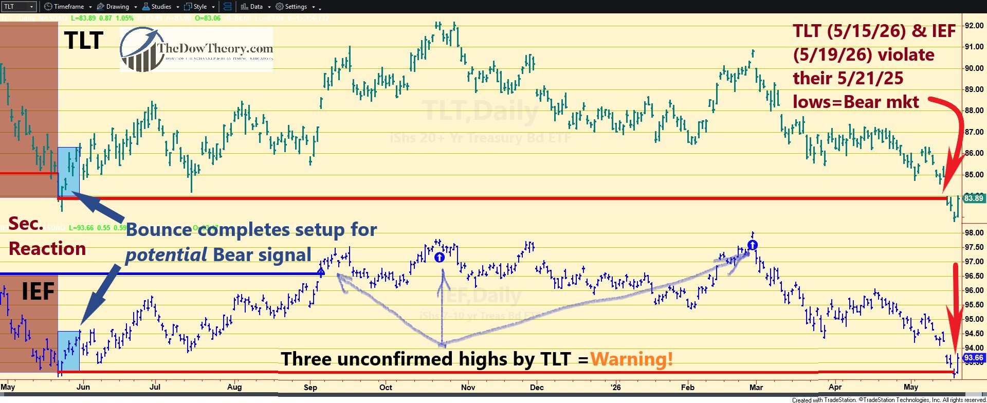
On 5/15/26, TLT violated its 5/21/25 secondary reaction lows. On 5/19/26, IEF confirmed by piercing its 5/21/25 secondary reaction lows. Confirmation means that a new primary bear market in bonds has been signaled.

The table below shows the price action that led to the primary bear market signal:

So, the primary and secondary trends are bearish now.

The following charts depict the latest price movements. Brown rectangles indicate the secondary (bearish) reaction opposing the ongoing primary bull market. Blue rectangles highlight the rally that completed the setup for a potential primary bear market (Step #3). Red horizontal lines mark the secondary reaction lows (Step #2). The blue horizontal lines show the bounce highs (Step #3). A breach of these peaks would signal a new primary bull market, though this scenario appears unlikely in the near term.

So, the situation is as follows: At the current juncture, a breakout on a closing basis by both TLT and IEF above their 4/4/25 closing highs (Step #1) would signal a new bull market. Until this breakout occurs, we consider bonds to be in a bear market.

B) Market situation if one sticks to the traditional interpretation requiring more than three weeks and 1/3 confirmed retracement to declare a secondary reaction.

As I explained in this post, the primary trend shifted to bullish on 4/4/25.

In this instance, the long-term application of the Dow Theory aligns with the shorter-term version, and hence the primary trend shifted to bearish on 5/19/26

Sincerely,

Manuel Blay

Editor of thedowtheory.com

 

Warning: Setup for potential primary bear market signal for Gold and Silver completed on 3/31/26

 Key price levels to watch are revealed in this post

Overview: GLD and SLV underwent a secondary reaction against the primary bull market. The recent price action completed the setup for a potential bear market signal on 3/31/26. Please mind the word “potential”, which implies that the primary bull market remains in force.

General Remarks:

In this post, I elaborate extensively on the rationale behind employing two alternative definitions to evaluate secondary reactions.

SLV refers to the Silver ETF. More information about SLV can be found HERE.
GLD refers to the Gold ETF. More information about GLD can be found HERE.

A) Market situation if one appraises secondary reactions not bound by the three weeks and 1/3 retracement dogma

As I explained in this post, the trend was signaled as bullish on 4/2/24.

From the 1/28/26 and 1/29/26 closing highs for SLV and GLD, respectively, both declined into 3/26/26. This pullback met the time and extent requirements for a secondary (bearish) reaction against the primary bullish trend.

Following the 3/26/26 lows, there was a 4-day rally that exceeded the Volatility Adjusted Minimum Movement (VAMM) on GLD and SLV (more about the VAMM HERE).

The table below gives you the relevant dates and prices:

So, now there are two options:

• If SLV and GLD surpass their 1/28/26 and 1/29/26 highs on a closing basis, Step #1 in the above table, the secondary reaction and setup for a potential bear market signal will be canceled.
• A primary bear market will be signaled if SLV and GLD break down below their 3/26/26 low ( Step #2).

The charts below illustrate recent price movements. The brown rectangles highlight the secondary reaction within the primary bull market. The small blue rectangles on the right show the early days of a rally that set up both ETFs for a potential primary bear market signal. The blue horizontal lines indicate the last recorded primary bull market highs that must be surpassed to reconfirm the bull market (Step #1). The red horizontal lines highlight the 3/26/26 lows (Step #2).

As of this writing, the primary trend is bullish, and the secondary one is bearish.

B) Market situation if one sticks to the traditional interpretation demanding more than three weeks and 1/3 confirmed retracement to declare a secondary reaction

As I explained in this post, the trend was signaled as bullish on 4/2/24.

In this instance, the long term application of the Dow Theory coincides with the shorter term version, so there was a secondary reaction against the primary bull market, and the setup for a potential bear market signal has been completed.

As of this writing, the primary trend is bullish, and the secondary one is bearish. 

Sincerely,
Manuel Blay

 Editor of thedowtheory.com 

 

Critical Juncture for Gold and Silver miners: Bear Market Signal One Step Away

 

In the meantime, the primary trend is still bullish, but it could change soon

Overview: GDX and SIL underwent a secondary reaction against the primary bull market. The recent price action completed the setup for a potential bear market signal on 3/25/26. Please mind the word “potential”, which implies that the primary bull market remains in force.

Gold and Silver are also in a secondary (bearish) reaction against the primary bull market but have not yet completed the setup for a potential primary bear market.

General Remarks:

In this post, I elaborate extensively on the rationale behind employing two alternative definitions to evaluate secondary reactions.

SIL refers to the Silver Miners ETF. More information about SIL can be found HERE.

GDX refers to the Gold Miners ETF. More information about GDX can be found HERE.

A) Market situation if one appraises secondary reactions not bound by the three weeks and 1/3 retracement dogma.  

As I explained in this post, the trend was signaled as bullish on 6/2/25.

From the 2/27/26 closing highs, both SIL and GDX dropped until 3/20/26. The decline met the time and extent requirement for a secondary (bearish) reaction against the primary bullish trend.

Following the 3/20/26 lows, there was a 3-day rally that exceeded the Volatility-Adjusted Minimum Movement (VAMM) on GDX. SIL also rallied, but percentage-wise did not exceed its VAMM. Please remember that we don’t require confirmation for the final rally that completes a bear (or bull) signal setup. More information is in this post.

The table below gives you the relevant dates and prices:

So, now there are two options:

1. If SIL and GDX surpass their 2/27/26 highs on a closing basis (Step #1 in the above table), the secondary reaction and setup for a potential bear market signal will be canceled.
2. A primary bear market will be signaled if SIL and GDX break down below their 3/20/26 lows (Step #2).

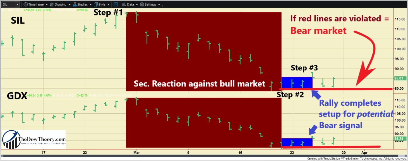
The charts below illustrate recent price movements. The brown rectangles highlight the secondary reaction within the primary bull market. The small blue rectangles on the right show the early days of a rally that set up both ETFs for a potential primary bear-market signal. The blue horizontal lines indicate the last recorded primary bull market highs that must be surpassed to reconfirm the bull market (Step #1). The red horizontal lines highlight the 3/20/26 lows (Step #2).

As of this writing, the primary trend is bullish, and the secondary one is bearish.

B) Market situation if one sticks to the traditional interpretation demanding more than three weeks and 1/3 confirmed retracement to declare a secondary reaction.

As I explained in this post, the trend was signaled as bullish on 6/2/25.

In this instance, the long-term application of the Dow Theory coincides with the shorter-term version, so there was a secondary reaction against the primary bull market, and the setup for a potential bear market signal has been completed.

As of this writing, the primary trend is bullish, and the secondary one is bearish.

Sincerely,

Manuel Blay

Editor of thedowtheory.com

 

The Four Industrial Revolutions: Why AI Changes Market Timing Forever

 

AI makes market timing more necessary than ever.

 

By George Morton, Ph.D

The stock market has always reflected the underlying economy, but not all economic transitions are created equal. Over the past 250 years, four industrial revolutions have reshaped how value is created, who captures it, and how fast leadership changes hands.

For investors, the key pattern is simple and uncomfortable: each revolution is arriving faster, scaling faster, and now—thanks to artificial intelligence (AI)—impacting productivity and earnings in years rather than decades.​

Steam power, electricity, and digital technology each followed a familiar script. A breakthrough in technology appeared, capital spending surged, adoption gradually spread, and only after long, uneven build‑outs did the real productivity gains show up in the data.

Investors had time to observe, adjust, and even recover from mistakes because the cycle from invention to broad economic impact ran 30–80 years. The Fourth Industrial Revolution, driven by AI, breaks that pattern. AI is compressing an entire industrial transition into a single market cycle, making when you are in or out of risk assets a far more consequential decision than in previous eras.​

First Industrial Revolution: Steam Power and Slow Motion Change

The First Industrial Revolution (roughly 1760–1840) was powered by steam engines that turned human and animal muscle into mechanized production. James Watt’s improvements in 1769 made steam engines efficient enough to move beyond mine drainage into textiles, metallurgy, and eventually railways, but the adoption curve was glacial by modern standards. It took about 80 years for steam to reach widespread penetration, as investors and entrepreneurs confronted high capital costs, scarce technical skills, and the need for entirely new infrastructure such as coal supply chains and machine tools.​

Crucially, the immediate payoff for the broader economy was modest. Total factor productivity growth from 1780 to 1830 averaged only about 0.3% per year, and steam contributed almost nothing to labor productivity before 1830. The real economic and market impact came much later—50 to 80 years after Watt’s patent—once complementary innovations in factories, transportation, and organizational models were in place. For investors in that era, “being late” by a decade or two did not mean missing the entire opportunity. The revolution unfolded slowly enough that mistakes could be corrected over a career, and long‑only, patient capital could still participate in the structural gains.​

Second Industrial Revolution: Electricity and the Age of Scale

The Second Industrial Revolution (1870–1914) was built on electricity, modern communications, and chemical synthesis. Practical dynamos and complete electrical systems turned power from a local asset—each factory maintaining its own steam plant—into a grid‑delivered service that could be flexibly deployed to lighting, motors, heating, and telecoms. Adoption accelerated: electricity reached roughly 50% penetration in about 40 years, half the time steam required. In the United States, household electrification rose from about 10% in 1903 to 68% by 1929.​

The impact on business models and capital markets was profound. Electricity enabled assembly lines, mass production, and the rise of huge integrated manufacturers and utilities. Yet even here, the productivity gains lagged the initial deployment by decades; firms needed time to redesign plants, reorganize workflows, and exploit the flexibility of electric motors instead of just swapping steam engines for electric ones. For investors, the key lesson is that the big winners—electrified mass producers, utilities, urban infrastructure plays—emerged over an extended period. Sector leadership changed, but the transition was still slow enough that buy‑and‑hold across broad industrials, rails, and utilities remained a viable strategy, albeit with large drawdowns across cycles.​

Third Industrial Revolution: Digital Technology and the Geography of Capital

The Third Industrial Revolution (1970–2000s) was driven by semiconductors, computing, and the internet. Microprocessors launched in the early 1970s, the internet coalesced around TCP/IP in the 1980s, and the World Wide Web opened global networks to non‑technical users in the 1990s. Digital technologies reached around 50% adoption in roughly 30 years, faster again than electricity. Computer costs fell about 19% per year from 1955 to 1987, and IT investment grew from less than 7% of total equipment spending in the 1950s to about half by the 2000s.​

Unlike earlier revolutions, the digital era directly reshaped capital markets themselves. The internet and enterprise software compressed supply chains, enabled offshoring, created entirely new sectors (software, platforms, e‑commerce), and delivered substantial value: manufacturing realized 1–2% cost savings, internet‑mature markets saw about a 500% increase in GDP per capita over 15 years, and digital‑savvy small firms generated twice the export revenue and employment growth of low‑internet peers. At the same time, the geography of winners shifted. Cities and companies that had thrived on Second‑Industrial‑Revolution density and heavy infrastructure began to lose ground to more flexible, digital‑native competitors. For investors, this era rewarded equity exposure but also introduced pronounced sector and style cycles—most famously the late‑1990s tech bubble and its aftermath—where timing and risk management started to matter more than in the steam and electricity eras.​

Fourth Industrial Revolution: AI, Three‑Year Adoption, and Immediate Productivity

The Fourth Industrial Revolution (2023–present) is powered by AI, machine learning, and autonomous systems that automate not just physical tasks but cognitive work itself. While AI research spans decades, mainstream adoption went vertically after late 2022. ChatGPT reached 100 million users in just two months, becoming the fastest‑growing consumer application in history. AI is expected to reach roughly 50% enterprise adoption in about three years—a 27‑fold acceleration versus steam’s 80‑year path. Current data from 2026 shows around 88% of organizations using AI in at least one business function and about 72% deploying generative AI specifically.​

This is not just faster adoption; it is a fundamental break in how quickly productivity gains arrive. Where steam and electricity needed 50–80 years to show up meaningfully in the data, AI is already delivering measurable improvements within 1–3 years of deployment. Studies of real‑world usage show AI reducing task completion times by around 80%—for example, cutting tasks that took 1.4 hours down to roughly 17 minutes. Aggregated across the economy, current‑generation AI models are estimated to add about 1.3–1.8 percentage points to annual US labor productivity growth over the coming decade, roughly doubling the pace experienced since 2019. That kind of uplift, arriving on a three‑year adoption curve, compresses decades of economic change into a single bull‑bear market sequence.​

For investors, this creates a new type of risk: not just the risk of missing an AI‑driven rally, but the risk that AI‑linked expectations—earnings, margins, multiples—get overextended and then violently repriced when reality temporarily undershoots the hype. The same infrastructure that accelerates AI deployment (cloud, data centers, models, capital) also accelerates repricing when sentiment turns.

New York City: A Cautionary Tale for Investors

The story of New York City across the industrial revolutions offers investors a real‑world case study of how seemingly permanent competitive advantages can evaporate when the underlying economic regime shifts. It is also a warning about what happens when capital allocators fail to anticipate or react to those shifts.​

The Glory Years: Second Industrial Revolution (1870–1970)

New York’s explosive growth during the Second Industrial Revolution reflected how electrical technologies rewarded density and concentration. Electric elevators enabled vertical construction—by 1930, Manhattan had 188 buildings exceeding twenty floors, including the Empire State Building’s 102 stories—packing white‑collar employment at densities impossible in the steam era. Electric streetcars and subways moved millions of workers daily, enabling the city to expand horizontally into Brooklyn, Queens, and the Bronx while maintaining Manhattan employment concentration.​

Electrical infrastructure transformed every dimension of urban life: electric lighting extended working hours and created vibrant nighttime entertainment districts; telegraph and telephone systems enabled Wall Street to coordinate global financial markets in real time, establishing New York as the world’s financial capital. The concentration created powerful network effects—deep labor markets, knowledge spillovers, specialized service providers—and by 1960, 128 Fortune 500 companies maintained headquarters in New York City, more than any other metropolitan area.​

For investors in that era, New York real estate, municipal bonds, utilities serving the city, and the corporations headquartered there were considered blue‑chip holdings. The city’s dominance seemed structural and durable.​

The Exodus: Third Industrial Revolution (1970–2000s)

The Third Industrial Revolution fundamentally undermined the competitive advantages that made New York dominant. When computing power became central to business models and digital networks enabled coordination without physical proximity, New York’s expensive real estate, aging infrastructure, high taxes, and congestion transformed from acceptable costs into unnecessary burdens.​

The corporate exodus accelerated during the 1970s through 1990s as companies relocated headquarters to suburban campuses and southern states offering lower costs and modern infrastructure. Between 1965 and 1976, New York City lost over 600,000 private sector jobs as manufacturing fled and corporate headquarters departed. Fortune 500 companies maintaining New York headquarters declined from 128 in 1960 to approximately 40 by 2000. The fiscal crisis of 1975, when the city nearly went bankrupt, symbolized how revolutionary technological change can undermine even seemingly unassailable competitive positions when economic fundamentals shift.​

For investors, New York’s decline was a multi‑decade bear market in city‑specific assets: commercial real estate values stagnated or fell, municipal bonds traded at distressed spreads, and the companies that stayed faced higher operating costs than competitors who left. Investors who treated NYC’s Second‑Industrial dominance as permanent paid a steep price.​

The Fourth Revolution: Return or Further Decline?

The Fourth Industrial Revolution presents ambiguous implications for New York and similar cities that dominated the Second Industrial Revolution. AI technologies could either favor continued dispersion—as cognitive work becomes fully location‑independent through AI‑enabled remote collaboration—or trigger renewed concentration if human creativity, judgment, and relationship skills complement rather than compete with machine intelligence.​

The dispersion scenario extends Third Industrial Revolution trends: AI‑enabled remote work eliminates remaining coordination advantages from physical presence; autonomous vehicles and delivery robots reduce logistics advantages of density; virtual reality meetings approach face‑to‑face quality while eliminating commuting. The concentration scenario envisions AI favoring density through different mechanisms: AI thrives on diverse data generated by dense urban interactions; AI development requires close collaboration among multidisciplinary teams; creative work that AI augments—strategic planning, business development, innovative problem‑solving—benefits from the knowledge spillovers and serendipitous encounters that dense environments facilitate.​

For investors, the New York story is a reminder that what looks like a durable, cash‑flow‑generating franchise in one industrial regime can become an over‑owned value trap in the next. Sectors, geographies, and business models that appear entrenched often prove fragile when the pace of technological change accelerates beyond the ability of existing institutions to adapt.​

Universities Across Four Revolutions: From Engine of Growth to Open Question

Universities have evolved alongside each industrial revolution, acting as critical enablers of growth—until now, when their role is becoming far less certain. For investors, the trajectory of higher education is a useful lens on how institutions that once drove transformation can themselves become structurally misaligned with a new economic regime.​

During the First Industrial Revolution, universities were still largely elite institutions focused on classical education, theology, and law. Technical skills for steam power and mechanized production were often learned through apprenticeships and on‑the‑job experience, not formalized engineering programs. The academy sat mostly adjacent to the new industrial economy rather than at its core.​

In the Second Industrial Revolution, that changed. The rise of electricity, chemicals, and large‑scale manufacturing drove the creation and expansion of research universities and technical institutes explicitly designed to produce engineers, chemists, and professional managers. In cities like New York, institutions such as Columbia and NYU became tightly coupled to industrial needs, training the workforce required by big factories, utilities, and vertically integrated corporations. Universities were, in effect, leveraged plays on the electrified industrial economy.​

The Third Industrial Revolution—computing and the internet—again reshaped demand, this time toward software engineering, computer science, and digital business models. Many universities adapted by adding CS departments, information systems programs, and business school tracks focused on technology and entrepreneurship. But the underlying model remained Second‑Industrial at its core: four‑year residential degrees, cost‑plus tuition pricing, and curricula built around relatively stable bodies of knowledge. As digital networks made information abundant and software skill cycles shorter, that model began to strain.​

The Fourth Industrial Revolution puts universities in an even more peculiar position. AI now provides instant access to expert knowledge, personalized tutoring, and continuously updated content at near‑zero marginal cost. In a world where AI adoption curves run three years instead of thirty, skills taught in freshman year can be obsolete before graduation, and credentials risk signaling past knowledge rather than current capability or learning velocity. Some universities are experimenting with lifelong learning, hybrid delivery, and a focus on uniquely human skills, but the traditional high‑cost, front‑loaded degree model is increasingly out of sync with AI’s pace.​

For investors, higher education is therefore a Fourth‑Revolution story that has not yet been fully priced or even fully told. Universities were clear beneficiaries of the Second and much of the Third Industrial Revolutions; in the AI era, they could evolve into powerful platforms for continuous reskilling—or become legacy institutions with declining pricing power and mounting balance‑sheet risk. As with New York City, the lesson is that institutions built for one technological epoch can look durable right up until a new general‑purpose technology exposes how rigid their economics really are.​

Why Timing Matters More Now Than Ever

When adoption and productivity unfold over 50–80 years, as they did with steam, investors can afford to be broadly right and approximately on time. Even electricity and digital technology, with 30–40 year adoption windows, gave markets years to absorb new leaders, rotate capital, and recover from over‑exuberant cycles. The AI era does not offer that luxury. A technology reaching 50% penetration in three years and delivering productivity and earnings impact within 1–3 years forces investors to confront a compressed cycle: leadership changes more quickly, thematic crowding builds faster, and drawdowns can erase several years of AI‑driven gains in a single primary bear market.​

That is why a disciplined, rules‑based timing framework—like The New Dow Theory’s indicators, which focus on confirmations and divergences across major indices and long‑term trend signals—becomes a core portfolio tool rather than a tactical curiosity. The goal is not to forecast every wiggle, but to distinguish primary bull and bear trends in enough time to materially reduce exposure during major downtrends and increase exposure when the odds again favor compounding.​​

In an environment where the Fourth Industrial Revolution is unfolding at a speed the market has never seen before, the history of the prior three revolutions is not just background—it is a warning. The pattern is familiar, but the clock has been reset, and investors who treat AI as “just another tech wave” risk discovering that this time, being early or late by a couple of years, is the difference between harvesting the revolution’s gains and financing them. Just as New York’s investors learned that Second‑Industrial dominance was not forever, today’s investors must recognize that AI‑era winners and losers will be determined on a timeframe that demands active, disciplined risk management rather than passive hope.

About the Author

This white paper synthesizes research of George Morton, Ph.D. from 150+ authoritative sources spanning academic journals, economic research institutions (McKinsey Global Institute, Boston Consulting Group, Deloitte, EY, PwC, World Economic Forum), federal research including the National Bureau of Economic Research and Federal Reserve Banks, industry analysts including Gartner and Forrester, and real-world enterprise implementations documented in case studies across manufacturing, financial services, healthcare, and legal services.

It builds upon the foundational quantitative analysis in “The Four Industrial Revolutions: An Exponential Acceleration in Technology Adoption and Economic Transformation” to provide strategic frameworks specifically designed for enterprise leaders navigating the compressed adoption timelines and fundamental business model transformations required by the AI revolution.

End of White Paper

© February 2026

All rights reserved. This document may be reproduced and distributed for educational and strategic planning purposes with appropriate attribution.